A popular game consists of finding the differences between 2 images. In this project we develop an application to do it automatically, using computer vision tools in Python (OpenCV and Scikit-image).
Introduction
In this first post, we build the main algorithm: i.e. finding the differences between two perfectly aligned images and displaying the result.
The steps are relatively simple:
- align the images (registration),
- do some blurring (of the typical size of a difference) to reduce the noise,
- compute a difference image,
- identify the difference areas on binary image,
- find the connected components
- display the location of the differences.
1. Image alignement
To do run the difference algorithm, we need the images to be perfectly aligned. Here we simply load 2 images that have been previsouly aligned (registered) as described in another post.
We do the usual library imports. diff_spotter is the final module containing all the routines for this project and can be found on GitHub.
## Preamble (importing the required libraries)
import cv2
import numpy as np
import matplotlib.pyplot as plt
from skimage.metrics import structural_similarity, mean_squared_error

import diff_spotter as ds

from importlib import reload

# for plotting
import matplotlib.pyplot as plt
plt.rcParams.update({'font.size': 25})

# plt.style.use('seaborn')
plt.style.use('seaborn-whitegrid')
plt.rc('pdf',fonttype=42)

import seaborn as sns
sns.mpl.rc('figure', figsize = (14, 8))
sns.set_context(
    'notebook', font_scale=2.5, rc={'lines.linewidth': 2.5})
We load the 2 images:
reload(ds)

# Read and display the 2 images (images have already been aligned)

# 1, 2, 3, 6, or 8
image_name = 'data/diff6'

img_a = cv2.imread(image_name+'_a_aligned.png')
img_b = cv2.imread(image_name+'_b_aligned.png')

ds.display_2img(img_a, img_b, file_name='plots/ex6.png')
2. Blurring
We blur the images to eliminate some of the noise. The kernel should be big enough to reduce noise but small enough to keep the high frequency of the differences (or we might miss them).
We expect the differences to be at least a few percents of the total size so the blurring kernel is about 2% of the width of the image.
kernel_size = int(img_a.shape[1]/50)

# must be odd if median
kernel_size += kernel_size%2-1

img_a_blurred = cv2.GaussianBlur(img_a, (kernel_size, kernel_size), 1.5)
img_b_blurred = cv2.GaussianBlur(img_b, (kernel_size, kernel_size), 1.5)

ds.display_2img(img_a_blurred, img_b_blurred, file_name='plots/ex6_blurred.png')
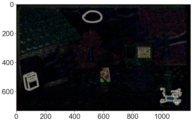
3. Image difference
We compute the actual difference between the 2 images (that is `img_a – img_b`). We use a spatial version of the Structural Similarity index algorithm to compute the difference (see https://en.wikipedia.org/wiki/Structural_similarity). It has the advantage of enhancing the spatially coherent image differences and is less prone to noise than a pure pixel-to-pixel difference. Note that we run morphological algorithms below to connect the components and that account for some of the parse result if we had run a simple pixel-to-pixel difference (to keep it mind if we accelerate the full process later).
# compute the spatial SSIM difference
ssim = True

if ssim:
    score, diff_ssim = structural_similarity(
        img_a_blurred, img_b_blurred,
        multichannel=True, full=True, gaussian_weights=True)
    # the diff is the opposite of the similarity
    diff = 1.0-diff_ssim

else:
    diff= cv2.absdiff(img_a_blurred, img_b_blurred)

# renormalise
diff = cv2.normalize(
    diff, None, alpha=0, beta=255, norm_type=cv2.NORM_MINMAX, dtype=cv2.CV_32F)
diff = diff.astype(np.uint8)

ds.display_img(diff, file_name='plots/ex6_ssim_diff.png')
4. Thresholding and noise removal
We first convert the color difference image to gray levels by taking the maximum among the color channels. We take this approach (instead of computing a gray-level image) because in some game, the difference is a change in color, therefore diluting the difference signal by a factor of 3 when if averaged over the color channels.
diff_gray = diff.max(axis=2)
ds.display_img(diff_gray)
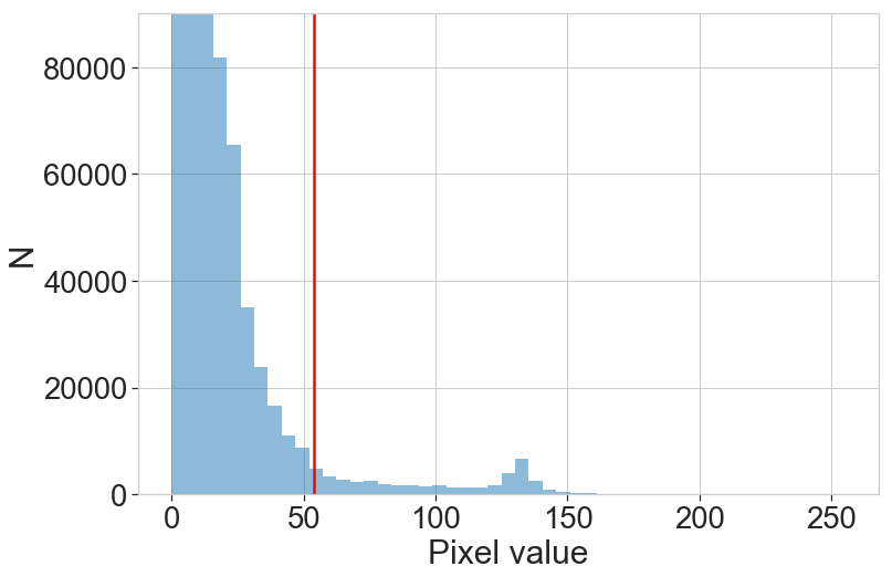
We compute the histogram of the gray difference image, we clearly see the bump around 130 that represents the pixels where the 2 images differ. We plot the threshold value to the 5% brightest pixels.
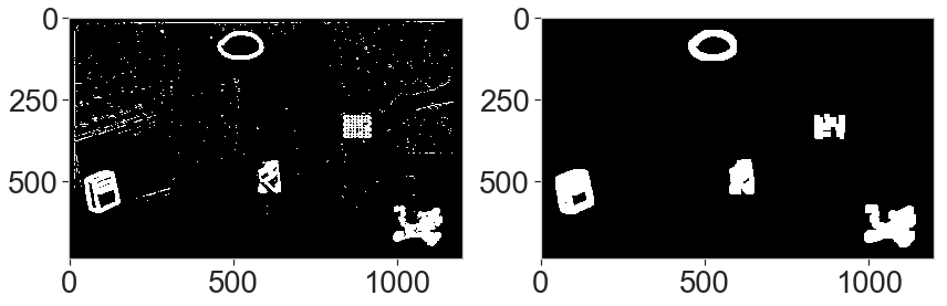
Next, we create a binary image and remove high-frequency noise to isolate large areas with significant difference. For this, we use the morphological operations “open” and “dilate” (see https://docs.opencv.org/trunk/d9/d61/tutorial_py_morphological_ops.html), to clean noise and connect nearby bright pixels.
The threshold value is chosen so that 5% of the brightest pixels are preserved. This corresponds roughly to the expected fraction of different pixels. So this parameter is crucial. A too low threshold will increase false detections (decreases precision) and a too high threshold will miss real detections (decreases recall).
tresh_quantile = 0.95

# threshold is set to 5% brightest pixels
min_thres = np.quantile(diff_gray, tresh_quantile)

# simple thresholding to create a binary image
ret, thres = cv2.threshold(diff_gray, min_thres, 255, cv2.THRESH_BINARY)

# opening operation to clean the noise with a small kernel
kernel = np.ones((3,3),np.uint8)
opening = cv2.morphologyEx(thres, cv2.MORPH_OPEN, kernel, iterations=3)

# and dilatation operation to increase the size of elements
kernel_dilate = np.ones((5,5),np.uint8)
diff_gray_thres = cv2.dilate(opening, kernel_dilate, iterations=2)

# Left: binary image, right after noise removal
ds.display_2img(thres, diff_gray_thres, file_name='plots/ex6_binary.png')
5. Component finding
We find the components (i.e. connected groups of pixels) and isolate them. We remove those suspected to be caused by the frame differences around the images, by removing long components exceeding the length of either half the width or half the height.
The components are sorted and we keep only the n largest. The default value is n=15, since the number of difference is between 5 and 10 and we want to be conservative in finding them: we allow a few false positives but want to capture all true differences (we maximize the recall).
# max number of differences
n_diff = 15

# detect connected components
retval, labels, stats, centroids = cv2.connectedComponentsWithStats(diff_gray_thres)

# remove outer border
components = []
for i, stat in enumerate(stats):

    x,y,w,h = stat[0:4]

    if (w > img_a.shape[0]*0.5) | (h > img_a.shape[1]*0.5):
        continue

    components.append(stat)

components = np.array(components)

# keep the 15 largest components
try:
    # sort based on the 4th column (the area)
    sorted_indices = components[:,4].argsort()

    # keep the 15 largest elements
    large_components = components[sorted_indices][-n_diff:]
except:
    pass

print(retval, large_components)
6 [[  830   296    95    77  5499]
 [  573   433    78   109  7042]
 [  448    39   149    97  7770]
 [   43   463   119   139 12104]
 [  983   572   159   130 13829]]
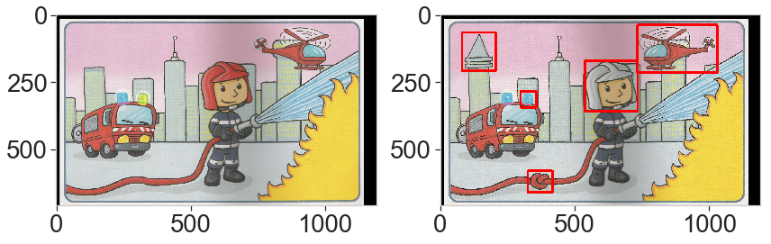
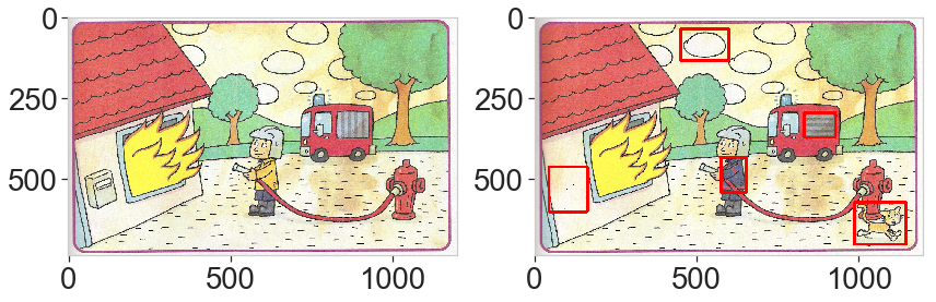
6. Difference highlights
Finally, we draw red rectangles around the selected components and overlay to the original image.
img_final = img_a.copy()
for component in large_components:
x,y,w,h = component[:4]
pt1 = (x,y)
pt2 = (x+w,y+h)
cv2.rectangle(img_final,pt1=pt1,pt2=pt2,color=(0,0,255), thickness=8)
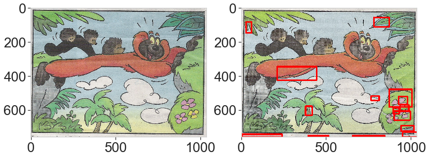
ds.display_2img(img_b, img_final, file_name='plots/ex6_final.png')
Full algorithm
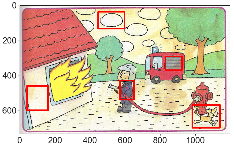
The function `find_difference` performs all the steps above. We show more examples below with some pitfalls and interesting results.
In this example, we miss the closed eyes of the hedgehog because of the cut on the large components that capture false differences in the image (caused by some shading during the scan process).
reload(ds)

image_name = 'data/diff1'
a = cv2.imread(image_name+'_a_aligned.png')
b = cv2.imread(image_name+'_b_aligned.png')
result = ds.find_differences(a, b, ssim=True, n_diff=15)

ds.display_2img(b, result, file_name='plots/ex1_final.png')
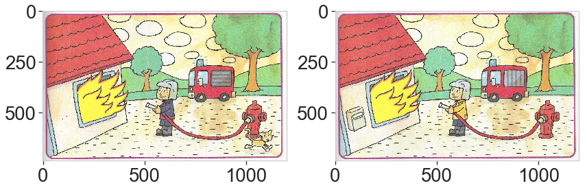
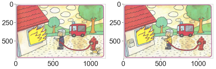
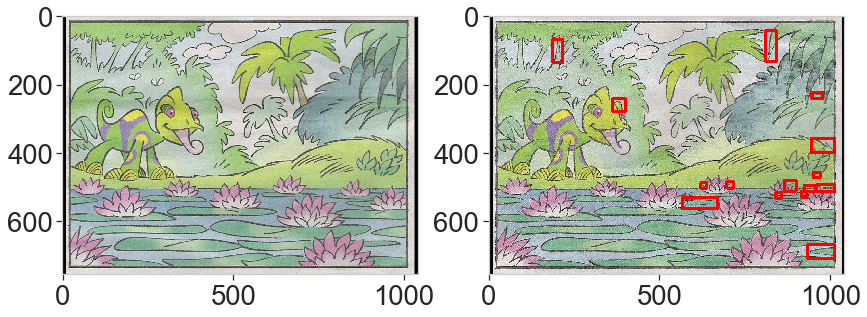
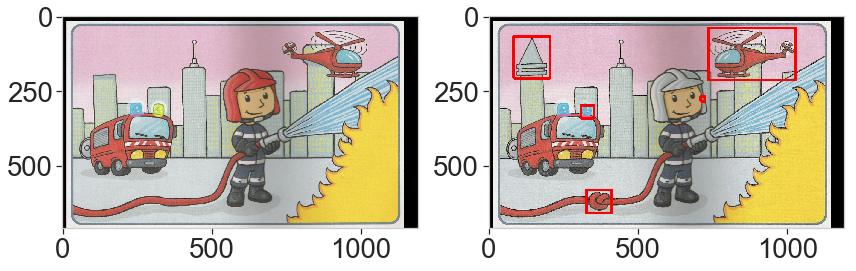
The two examples below have a high recall (we capture all the difference) but not perfect precision as we wrongly detect some false differences.
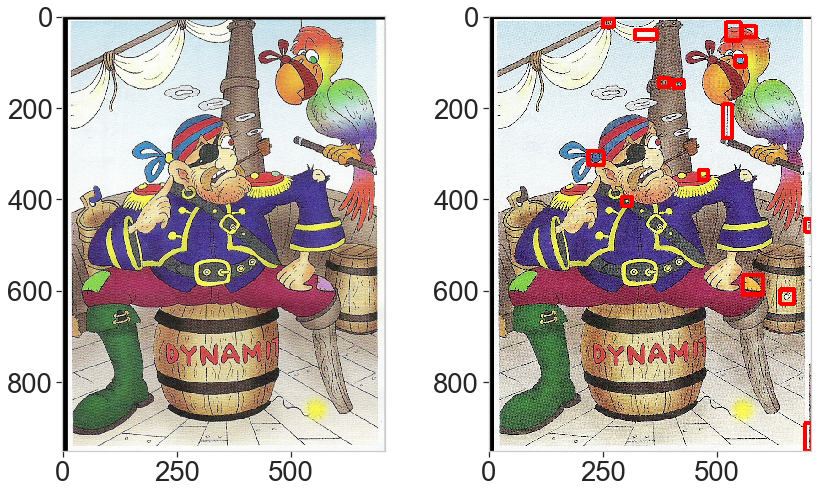
This last example is interesting. The differences are obvious but one is almost overlooked (the helmet) with the default parameters. This is due to the threshold limit: because the total area is very large, the change in color of the helmet is excluded from the selected brightest pixels. Lowering down the threshold by picking the 90% percentile solves the problem.
result = ds.find_differences(a, b, tresh_quantile=0.90, n_diff=5)