
Following the extension of the family, we decided to buy a new and bigger car, and hence to sell the old one (an Audi A3 sportsback). There exists online ressources to evaluate the price of used cars on the market (Eurotax for the Swiss market) but the car was too old to be listed (over 12 years) so I attempted to evaluate the price of my car based on the market, using web scraping and a bit of machine learning.
It turned out that I sold the car much below the market price due to a technical problem in the engine that I had first overlooked. But the exercise was nevertheless interesting and very useful to have a first idea of the price. It is also worth mentioning that a professional friend of mine helped me during the selling process. The business experience is often superior in these situations.
The adopted strategy consists in 3 steps:
- first acquire some data online including the price and the car characteristics
- build a pricing model using machine learning
- evaluate the price of my car given its characteristics
Preamble
As usual we import the necessary libraries.
# system libraries
import os
import sys
import re
from datetime import date, datetime, timedelta
import numpy as np

# for data handling
import pandas as pd

# for web scraping
import requests
from bs4 import BeautifulSoup

# for plotting
import matplotlib.pyplot as plt
plt.rcParams.update({'font.size': 25})

# plt.style.use('seaborn')
plt.style.use('seaborn-whitegrid')
plt.rc('pdf',fonttype=42)

import seaborn as sns
sns.mpl.rc('figure', figsize = (14, 8))
sns.set_context(
    'notebook', font_scale=2.5, rc={'lines.linewidth': 2.5})
Data acquisition
To obtain the data I need, I get the data from a swiss selling items web site, focusing on the used car ads. I had several choices but I found one site that was relatively easy to analyse while having many ads (about 200k used car ads).
As usual the goal is to find the best compromise between getting as much data as possible while saving ressources in time and computing power (from both sides of the server and the client). The approach I choose is to get the data from the ad preview, which already contains the most critical pieces of information (such as car model, price, age and kilometers).
Data exploration
The scraping has been done twice. The first time on June 22nd and one week later. The goal is to see which typical ads have disappeared in the interval (i.e. if they were sold rapidely).
Import data
data_dir = 'data'
# read csv files
df_1 = pd.read_csv(data_dir+'/22.06.2019_all.csv', index_col='item_id')
df_2 = pd.read_csv(data_dir+'/29.06.2019_all.csv', index_col='item_id')

# merge the two
df_ads = df_1.join(
    df_2['age_ad_days'], rsuffix='_2', how='left', on='item_id')

# create a new column: True if it disa
select = (df_ads['age_ad_days_2'].isnull()) & (df_ads['date']>='2019-06-21')
df_ads['less_than_a_week'] = select
df_ads = df_ads.drop('age_ad_days_2', axis=1)

# Display numbers
print('Total: {0}. Disappeared in 1 week: {1}'.format(len(df_ads), sum(select)))
Total: 232642. Disappeared in 1 week: 1176
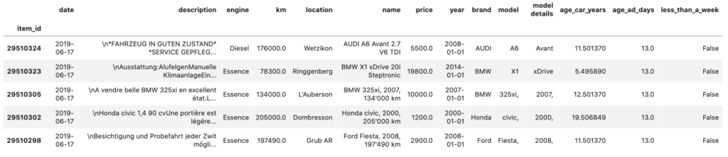
df_ads.drop('link', axis=1).head()
Cleaning
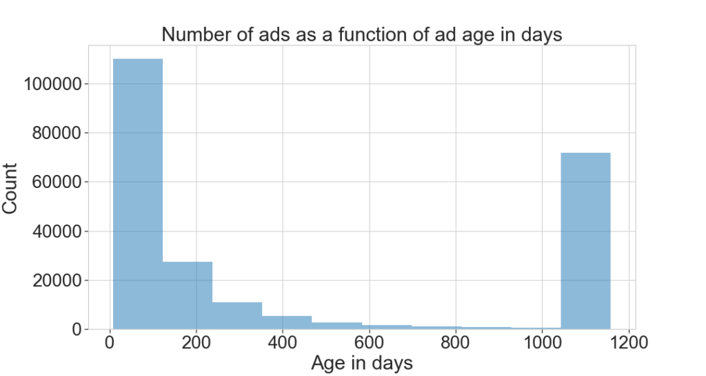
We take a quick look at the data and clean what’s necessary. Here we see that a number of ads are over 1000 days old and some have no valid date. This may correspond to promoted ads. We remove them. We also remove prices over CHF 1M.
Identically, some ads have a very high number of kilometers.
In total we get rid of 36% of ads.
fig, ax = plt.subplots(figsize=(15,8))

ax.hist(
    df_ads['age_ad_days'].dropna(), alpha=0.5,
    label='All', density=False) #, bins=np.linspace(10,50))
ax.set_xlabel('Age in days')
ax.set_ylabel('Count')
ax.set_title('Number of ads as a function of ad age in days')

fig.savefig('figures/ad_age_distribution.png')
# cleaning
select = df_ads['age_ad_days'] > 0
select &= df_ads['age_ad_days'] < 1000
select &= df_ads['price'] < 1.e6
select &= df_ads['price'] > 0
select &= df_ads['km'] > 0
select &= df_ads['km'] < 2.e5
df_ads_clean = df_ads[select]

# how much is it dropped?
N = len(df_ads)
N_clean = len(df_ads_clean)

#(len(df_ads)-len(df_ads_clean))/len(df_ads)

print('N: {}, N(clean): {} , dropped fraction: {:.2f}%'.format(
    N, N_clean, 100.*(N-N_clean)/N))
N: 232642, N(clean): 149590 , dropped fraction: 35.70%
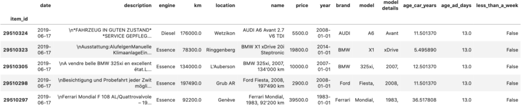
df_ads_clean.drop('link', axis=1).head()
Price distribution
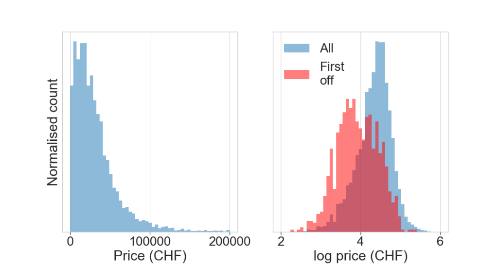
The price is our target to estimate. We take a look at its distribtution. Interstingly, the price distribution is roughly log-normal, i.e. the logarithm of it normal, and hence skewed towards higher values. The median price is CHF 28’800.
We overplot the distribution of ads that disappeared within 1 week in red, “first off” the list. We see a significant decrease in price. The median price is CHF 8000. This is consistent with the fact that cheaper cars are sold faster.
fig, ax = plt.subplots(1,2, figsize=(15,8), sharey=False)

ax[0].hist(
    df_ads_clean['price'], alpha=0.5,
    label='All', density=True, bins=np.linspace(0,2.e5))
ax[0].set_xlabel('Price (CHF)')

ax[1].hist(
    np.log10(df_ads_clean['price']),density=True, alpha=0.5,
    label='All', bins=np.linspace(2,6))

select = df_ads_clean['less_than_a_week']
ax[1].hist(
    np.log10(df_ads_clean[select]['price']), alpha=0.5,
    label='First\noff', density=True, bins=np.linspace(2,6), color='red')

ax[1].set_xlabel('log price (CHF)')

ax[0].set_yticks([])
ax[1].set_yticks([])

ax[0].set_ylabel('Normalised count')

ax[1].legend()

print(df_ads_clean['price'].median(), df_ads_clean[select]['price'].median())

fig.savefig('figures/price_distribution.png')


None
24800.0 8000.0
Features
Next, we explore here the distribution of features and the correlation between them. First we pick a number of features and see how the price depends on them, then we look at the distribution of the features.
attributes = ['km', 'age_car_years',  'age_ad_days']
# fig, ax = plt.subplots(figsize=(4,4))
n_i, n_j = 1, 3
fig, ax = plt.subplots(
    n_i, n_j, figsize=(15, 6), sharey = True)
# plot price vs attribute
for k, a in enumerate(attributes):
    df_ads_clean.plot.scatter(
        x=a, y='price',
        ax=ax[k],
        s=10, alpha=0.1)
fig.tight_layout()

fig.savefig('figures/price_vs_features.png')


fig, ax = plt.subplots(
    n_i, n_j, figsize=(15, 6), sharey = True)

# plot price vs attribute
for k, a in enumerate(attributes):
    df_ads_clean[a].plot.hist(
        ax=ax[k], alpha=0.5, logy=False)
    ax[k].set_xlabel(a)

fig.tight_layout()

# ax=ax[k%n_i, k//n_i],
# do not plot axes with no data
#for k in range(len(attributes),n_i*n_j ):
#    ax[k%n_i, k//n_i].axis('off')

fig.savefig('figures/features_distribution.png')

None
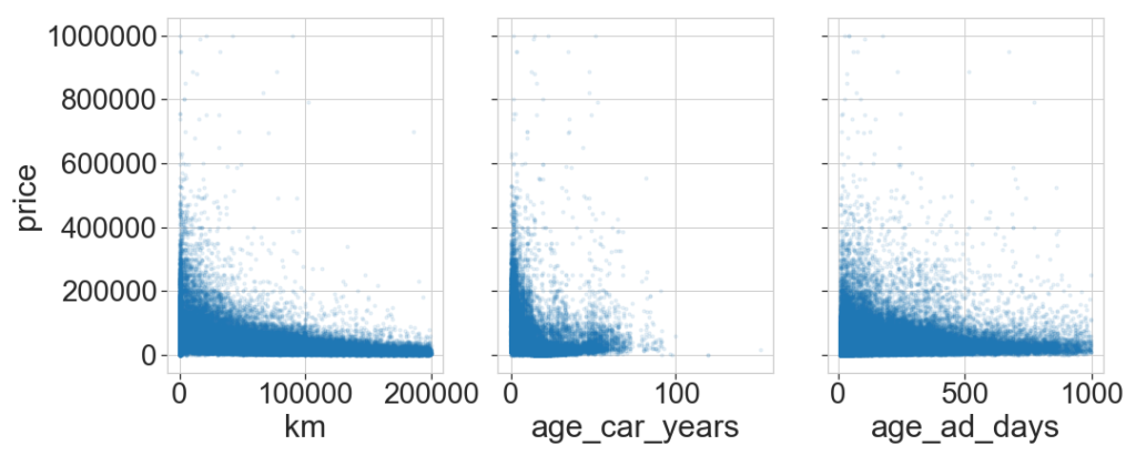
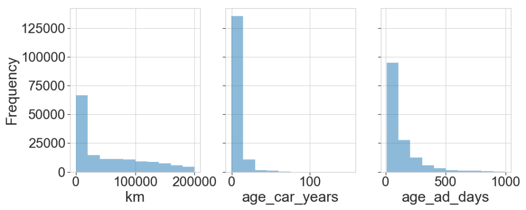
Most cars have few kilometers and are relatively new. As expected the price increases with low km and small age.
Price modelling
We will now focus on a specific model, i.e. the one we attempt to model the price, an Audi A3.
Selection of the car model
We apply a number of filters on the brand, model and model details. As the text form is free, we are flexible in the search term.
# Brand and model
select = df_ads_clean['brand'].fillna('').str.contains('Audi|AUDI|audi')
select &= df_ads_clean['model'].fillna('').str.contains('A3|a3')

# Select specifically the sportsback (5 doors) models
select &= \
    df_ads_clean['model details'].fillna('').str.contains('Sportback|sportback')\
    |df_ads_clean['description'].fillna('').str.contains('Sportback|sportback')\
    |df_ads_clean['name'].fillna('').str.contains('Sportback|sportback')

# Engine type
select &= \
    df_ads_clean['model details'].fillna('').str.contains('TDI')\
    |df_ads_clean['description'].fillna('').str.contains('TDI')\
    |df_ads_clean['name'].fillna('').str.contains('TDI')

# We exclude new cars
select &= df_ads_clean['km'] > 1000.
select &= df_ads_clean['age_car_years'] > 1

df_Audi_A3 = df_ads_clean[select].copy()

print(sum(select))
247
Feature selection
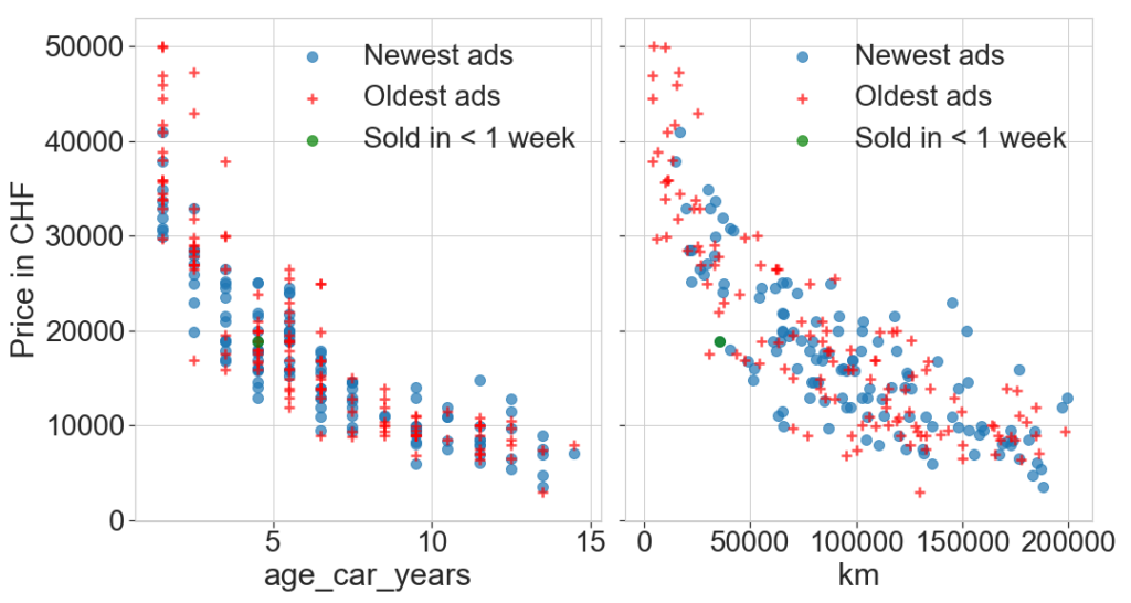
We now plot the price as a function of km and age of the car for the Audi A3. We observe the same trends as before, i.e. that the price increases with decreasing km and age, but much clearly than with the full population (See above).
We then split the sample in two, above and below the median ad age (50 days). The former is plotted in blue (“newest”) whereas the latter is plotted in red (“oldest”). WHerease no significant trend is visible a priori on the plot, when we look at the mean price, however, oldest ads have a higher value, and both the ratio mean(price)/mean(age) and the ratio mean(price)/mean(km) are higher (around 30%) for old ads than new ads.
The two features km and car age will be our machine learning primary parameters to model the price. Since the price is an exponentially decreasing function of both parameters, it’s clear that some transformation will ease the modelling (see next section).
fig, ax = plt.subplots(1, 2, figsize=(15,8), sharey=True)

select = df_Audi_A3['age_ad_days'] > df_Audi_A3['age_ad_days'].median()

df_Audi_A3[~select].plot.scatter(
    marker='o', x='age_car_years',
    y='price', ax=ax[0], s=100, alpha=0.7, label='Newest ads')
df_Audi_A3[~select].plot.scatter(
    marker='o', x='km',
    y='price', ax=ax[1], s=100, alpha=0.7, label='Newest ads ')

print('Median age of the ad in days', df_Audi_A3['age_ad_days'].median())

means_newest = df_Audi_A3[~select].mean()
means_oldest = df_Audi_A3[select].mean()

print('Newest:\n', means_newest)
print('Oldest:\n', means_oldest)

print('Price to age ratio newest: {:.2f}'.format(means_newest['price']/means_newest['age_car_years']))
print('Price to age ratio oldest: {:.2f}'.format(means_oldest['price']/means_oldest['age_car_years']))

print('Price to km ratio newest: {:.2f}'.format(means_newest['price']/means_newest['km']))
print('Price to km ratio oldest: {:.2f}'.format(means_oldest['price']/means_oldest['km']))

# print('Price to km and age ratio newest: {:.3f}'.format(means_newest['price']/means_newest['km']/means_newest['age_car_years']))
# print('Price to km and age ratio oldest: {:.3f}'.format(means_oldest['price']/means_oldest['km']/means_oldest['age_car_years']))

if select.any():
    df_Audi_A3[select].plot.scatter(
        x='age_car_years', y='price', ax=ax[0], s=100, alpha=0.7,
        marker='+', c='red', label='Oldest ads')
    df_Audi_A3[select].plot.scatter(
        x='km', y='price', ax=ax[1], s=100, alpha=0.7,
        marker='+', c='red', label='Oldest ads')

select = df_Audi_A3['less_than_a_week']
if select.any():
    df_Audi_A3[select].plot.scatter(
        x='age_car_years', y='price', ax=ax[0], s=100, alpha=0.7,
        marker='o', c='green', label='Sold in < 1 week')
    df_Audi_A3[select].plot.scatter(
        x='km', y='price', ax=ax[1], s=100, alpha=0.7,
        marker='o', c='green', label='Sold in < 1 week')

# Aestetics
ax[0].set_ylabel('Price in CHF')

fig.tight_layout()

fig.savefig('figures/price_vs_age_and_km.png')
Median age of the ad in days 58.0
Newest:
 km                   97928.564516
price                16873.500000
age_car_years            6.537251
age_ad_days             29.209677
less_than_a_week         0.008065
log_age_car_years        0.747052
log_km                   4.924243
dtype: float64
Oldest:
 km                   86942.609756
price                19864.528455
age_car_years            6.073728
age_ad_days            172.414634
less_than_a_week         0.000000
log_age_car_years        0.696783
log_km                   4.789348
dtype: float64
Price to age ratio newest: 2581.13
Price to age ratio oldest: 3270.57
Price to km ratio newest: 0.17
Price to km ratio oldest: 0.23
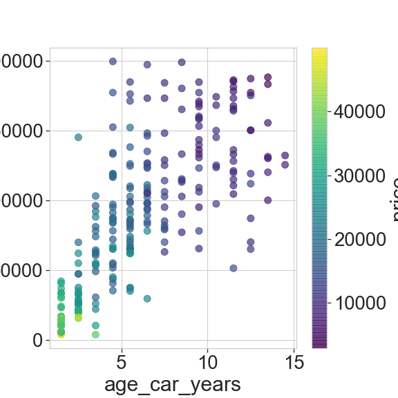
We also plot the km as a function of car age. As expected the former increases with the latter. What’s interesting is to see the high scatter for high values, and that’s what interests us given that our car is old but with relatively few km, so we will see to model it properly to see whether it increases its value.
And to start analysing we set the point color as the price. We clearly see the strong dependence on age. However, the km dependence seems to be less promominent. We will probably find that the age is the primary factor to estimate the price.
fig, ax = plt.subplots(figsize=(8,8))

df_Audi_A3.plot.scatter(
    marker='o', x='age_car_years', y='km',
    ax=ax, s=100, alpha=0.7, c='price', cmap='viridis')

fig.savefig('figures/km_vs_age.png')

None
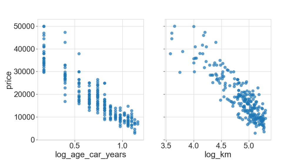
Feature transformation
Since the price is an exponentially decreasing function of age and km, we apply a logarithmic transformation of the features (a particular case of cox-box transformation):
df_Audi_A3['log_age_car_years'] = df_Audi_A3['age_car_years'].apply(np.log10)
df_Audi_A3['log_km'] = df_Audi_A3['km'].apply(np.log10)

fig, ax = plt.subplots(1, 2, figsize=(15,8), sharey=True)

df_Audi_A3.plot.scatter(
    marker='o', x='log_age_car_years', y='price', ax=ax[0], s=100, alpha=0.7)
df_Audi_A3.plot.scatter(
    marker='o', x='log_km', y='price', ax=ax[1], s=100, alpha=0.7)

fig.savefig('figures/price_vs_age_and_km_log.png')

fig.tight_layout()
Price modelling
We finally apply a machine learning algorithm to model and predict the price. We test a linear, a random forest, and a support Vector machine (SVN) models. To test the model, we compute a mean square error (root squared) and the score provided by the model object (r^2 score in the linear case) on a “test” sample kept aside when training the model.
import sklearn

from sklearn.linear_model import LinearRegression
from sklearn.naive_bayes import GaussianNB, BernoulliNB, MultinomialNB
from sklearn import svm
from sklearn.neural_network import MLPRegressor
from sklearn.ensemble import RandomForestRegressor, AdaBoostRegressor
from sklearn import metrics
# functions
def split_data(X, y):
    """ Split the data assuming
    training: 80%, test: 20% """

    X_train, X_test, y_train, y_test = \
    sklearn.model_selection.train_test_split(
        X, y, test_size=0.20)

    return X_train, X_test, y_train, y_test

def fit_data(df, model, n_iter=100):

    # perform multiple regression
    attributes = ['log_age_car_years', 'log_km']

    X = df[attributes]
    y = df['price']

    error = np.zeros(n_iter)
    score = np.zeros(n_iter)
    for n in range(n_iter):
        X_train, X_test, y_train, y_test = split_data(X, y)

        model.fit(X_train, y_train)

        y_test_predict = model.predict(X_test)
        y_train_predict = model.predict(X_train)

        error[n] = np.sqrt(metrics.mean_squared_error(y_test, y_test_predict))
        score[n] = model.score(X_test, y_test)


    return error.mean(), error.std(), score.mean(), score.std()
# Test several models
models ={
    'Linear': LinearRegression(normalize=True, fit_intercept=True),
    'Random Forest': RandomForestRegressor(n_estimators=20),
#    'Neural network': MLPRegressor(hidden_layer_sizes=(10,)),
    'SVM': svm.SVC(gamma='scale'),
}

for model_name in models.keys():
    error, error_std, score, score_std = fit_data(df_Audi_A3, models[model_name])

    error_str = 'error: {:.2f} (+/- {:.2f})'.format(error, error_std)
    score_str = ', score: {:.2f} (+/- {:.2f})'.format(score, score_std)
    print('{:20}'.format(model_name)+error_str,score_str)
Random Forest       error: 3699.78 (+/- 530.80) , score: 0.85 (+/- 0.04)
Linear              error: 3249.61 (+/- 503.02) , score: 0.88 (+/- 0.04)
SVM                 error: 11188.55 (+/- 1667.60) , score: 0.01 (+/- 0.01)
The linear model performs best. The random forest is also quite good whereas the SVM model is significantly worse than the other 2.
Audi price
In this final step, we predict the price of our Audi, given that it’s 13 years old and has 96’000 km.
We have seen previously that the model predictions were relatively noisy even for one model. Since the training process is fast, we randomise the process to evaluate the typical price variation due to the machine learning process. To do so, we repeat the training and prediction 100 times, then computing the mean and standard deviation of the price.
For the linear model, the predicted price from the market is CHF 9300 (+/- 170).
def estimate_price(df, model, n_iter=100):

    # perform multiple regression
    attributes = ['log_age_car_years', 'log_km']

    X = df[attributes]
    y = df['price']

    log_x = np.log10([13.0, 96000.])

    price = np.zeros(n_iter)
    for n in range(n_iter):
        X_train, X_test, y_train, y_test = split_data(X, y)
        model.fit(X_train, y_train)

        price[n] = model.predict([log_x])

    return price.mean(), price.std()
for model_name in models.keys():
    price, price_std = estimate_price(df_Audi_A3, models[model_name])

    price_str = 'price: {:.2f} (+/- {:.2f})'.format(price, price_std)
    print('{:20}'.format(model_name)+price_str)
Random Forest       price: 8175.42 (+/- 613.93)
Linear              price: 9281.72 (+/- 172.44)
SVM                 price: 11610.00 (+/- 2146.14)
Finally estimate using oldest and newest ads as training. The linear model is similar. The svm and random forest feature significant higher prices when trained with oldest ads.
newest = df_Audi_A3['age_ad_days'] > df_Audi_A3['age_ad_days'].median()
oldest = df_Audi_A3['age_ad_days'] <= df_Audi_A3['age_ad_days'].median()

for model_name in models.keys():
    price, price_std = estimate_price(df_Audi_A3[newest], models[model_name])

    price_str = 'price: {:.2f} (+/- {:.2f})'.format(price, price_std)
    print('{:20}'.format(model_name)+price_str)

for model_name in models.keys():
    price, price_std = estimate_price(df_Audi_A3[oldest], models[model_name])

    price_str = 'price: {:.2f} (+/- {:.2f})'.format(price, price_std)
    print('{:20}'.format(model_name)+price_str)
Random Forest       price: 7489.03 (+/- 746.82)
Linear              price: 9195.37 (+/- 270.22)
SVM                 price: 9010.00 (+/- 705.62)
Random Forest       price: 10228.56 (+/- 589.40)
Linear              price: 9159.41 (+/- 215.46)
SVM                 price: 12684.00 (+/- 1786.55)
# log_x = np.log10([13.0, 96000.])
# models['Linear'].predict([log_x])
Feature importance
A final interesting thing to do is explore the importance of features, which can be done with random forest. Since part of randomisation process is done on the feature, the algorithm is able to estimate which feature gives the most information.
Here we see that the age is the most important feature, contributing to almost 70% of the fitting process, whereas the number of km only contribute to only 30%.
attributes = ['log_age_car_years', 'log_km']

importances = models['Random Forest'].feature_importances_
std = np.std([tree.feature_importances_ for tree in models['Random Forest'].estimators_],
             axis=0)

indices = np.argsort(importances)[::-1]

# Print the feature ranking
print("Feature ranking:")

X = df_Audi_A3[attributes]
for f in range(X.shape[1]):
    print("%d. feature %d (%f)" % (f + 1, indices[f], importances[indices[f]]), X.columns[f])
Feature ranking:
1. feature 0 (0.669670) log_age_car_years
2. feature 1 (0.330330) log_km
Conclusion
To conclude:
- choice of model: linear on log-transformed features seems to be the most robust
- best estimation: CHF 9’300
- most import feature: age of the car
- oldest ads have a higher price (probably meaning the price is too high)
The fact that the age of the car is the most important feature to estimate the price means that owning a car we don’t use really is a bad idea. Indeed, after some years, whether we used a car or not, its price will still significantly decreases. And that is the case here, although the number of kilometers is relatively low, it didn’t help to give it a better price on the market.
Also, it would be interesting to investigate a bit more, but it seems evident there is a minimum number of kilometers under which renting a car from time to time is more profitable than owning or leasing a car.